CT-to-Report Does NOT Work, Yet

TL;DR

This is a collection of studies on the task of RRG (“CT DICOMs in, Report out”).

• We finally see a good-sized (~50k) dataset with reports , which further attracts more “annotations”
• None of the direct report generation methods are really working
• Even worse, The numbers DON’T MATCH across papers (CT2Rep)
  • which shows a lack of a consistent benchmark
  • perhaps the new challenge will redeem the problem ¹

CT-CLIP

NOTE: The paper and dataset were first published in 03/24, but the figure is drawn from the v3 version in 04/25.

Takeaway

• good amount CT data with labels ²
• native, whole-CT abnormalities classification DOES NOT work

Dataset (CT-RATE)

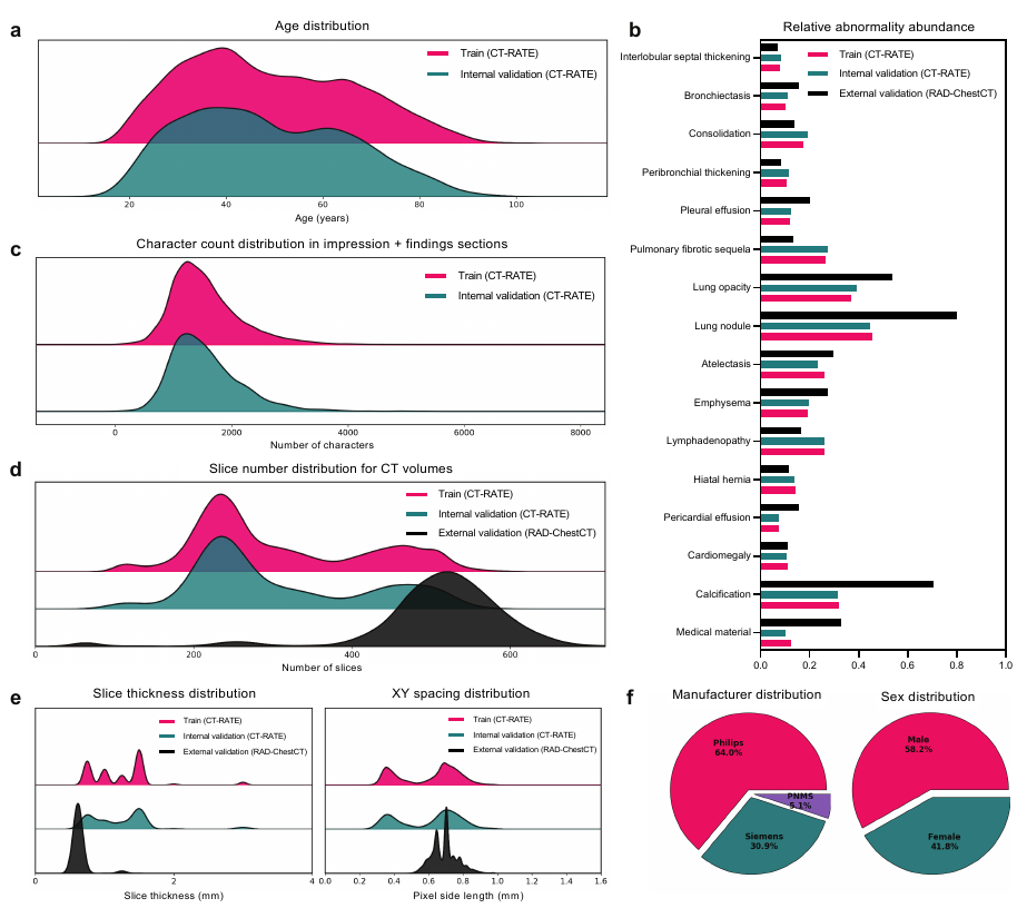
• 50,188 non-contrast 3D chest CT volumes (series_id) from 25,692 distinct CT experiments (study_id) conducted on 21,304 unique patients (patient_id).
• with reports and parsed into 18 distinct types of abnormalities
• with extended metadata

Abnormality Distribution

1. Medical material
2. Arterial wall calcification
3. Cardiomegaly
4. Pericardial effusion
5. Coronary artery wall calcification
6. Hiatal hernia
7. Lymphadenopathy
8. Emphysema
9. Atelectasis
10. Lung nodule
11. Lung opacity
12. Pulmonary fibrotic sequela
13. Pleural effusion
14. Mosaic attenuation pattern
15. Peribronchial thickening
16. Consolidation
17. Bronchiectasis
18. Interlobular septal thickening

Method and Results

• Extract labels from reports with fine-tuned RadBERT
• CT-ViT with
  • patch size of 20 × 20 × 10
  • normalized spacing of 0.75mm x 0.75mm x 1.5mm
  • normalized resolution of 480 × 480 × 240
  • ending up with 24^3 = 13,824 patches compressed to a 512-channel embedding before the text embedding
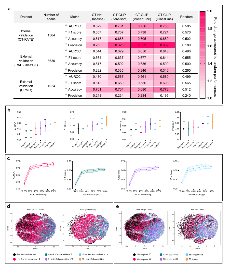
• several strategies, such as supervised, linear probing, CT-CLIP, etc.
• Performance is better than random but NOT usable; even worse, it GENERALIZES POORLY

RadGenome-ChestCT

Takeaway

More annotations for CT-RATE - segmentation, hierarchical structure identities, and VQA³

Method

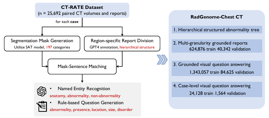
New annotations added for the CT-RATE dataset

• universal segmenter SAT⁴: whole body segmentation of 197 categories
• LLM and NER parsing: GPT-4 annotated hierarchical structure: Breaks each report into an anatomically-hierarchical tree and align every sentence to the matching mask region.
• Rule-based template: Generates grounded VQA pairs that ask about abnormality presence, location, size, etc.

CT2Rep

Takeaway

• A good first-effort attempt; has been used as a baseline for comparison for CT RRG

Method

• First direct CT → image encoder → text decoder to generate a report

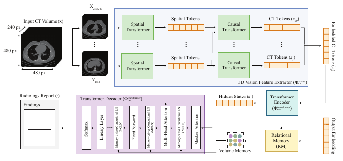
• similar to CT-CLIP preprocessing, but patch size of 12x24x24, ending up with 20^3 = 8,000 vision embeddings
• Added a follow-up setting, CT2RepLong, but the results did not get better…

Result

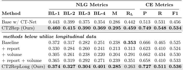
• NOTE: RepLong reports lower aggregate precision and recall but a higher aggregate F1. Separate macro-averaging can produce this pattern, so it is not by itself proof of an error. The paper’s averaging convention needs to be checked before comparing these columns.

Detailed Result

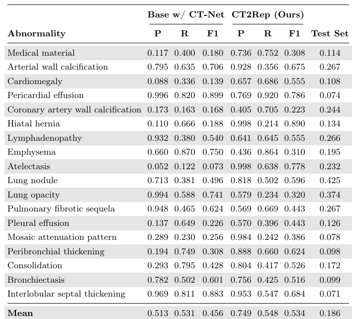
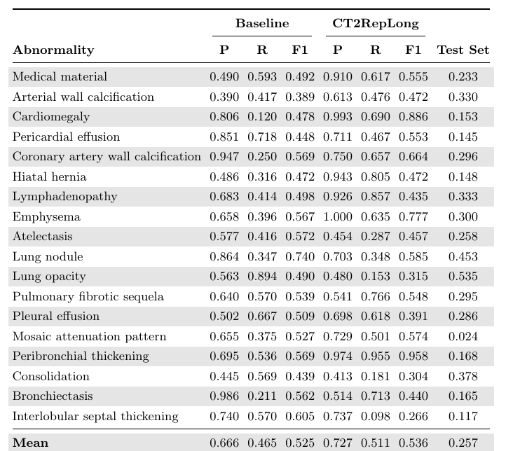
• The per-label table also warrants clarification: for medical material, Table 2 reports precision 0.736, recall 0.752, and F1 0.308. If these come from one confusion matrix, F1 should be approximately 0.744. Separate averaging could change that relationship; the table alone does not establish how these values were aggregated.

CT-AGRG

Takeaway

• A native baseline to start with
• CT-Net with CNN architecture > CT-ViT with Transformer architecture
  • Aligns with my expectation: ViT is limited due to the current setting (full-size CT → sparse supervision)

Method

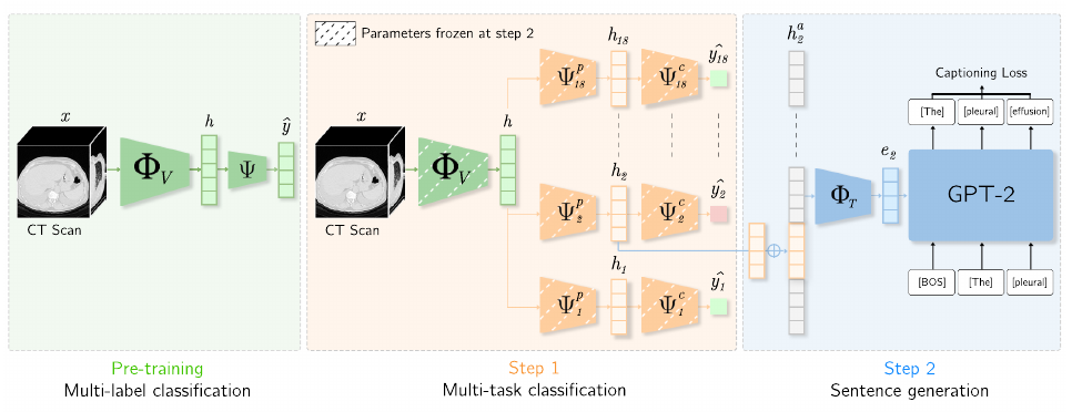
• Use a visual encoder to train on supervised classification first, then integrate it with a small GPT-2 for report generation
  • multi-label → multi-task embedding → report sentence

result

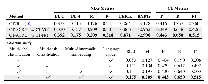
Detailed Result

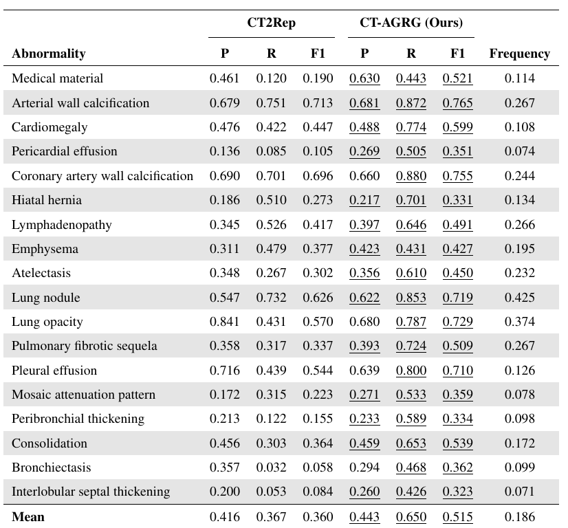
The results of CT2Rep are COMPLETELY DIFFERENT from what is reported in the original paper, though the frequencies are the SAME suggesting the dataset is the same

Version note: The detailed table below is Table 2 in arXiv:2408.11965v3. The comparison here is pinned to that version; later revisions may differ.

CT-Agent

Takeaway

• First attempt? To integrate a whole CT volume into an LLM

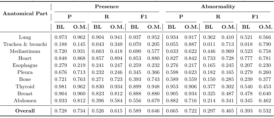
• Interesting, regionally prompted analysis reveals that the MLLM CANNOT identify some organs well

Method

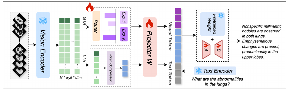
• frozen 2D CLIP (ViT-B/16): as vision encoder, each image is 256 tokens = a total of 240 (slice) x 256 (num_token) x 1024 (emb_dim) tensor to start with
• Global Token Aggregation (GTA): compresses the volume into 256 x 1024 global embedding
• Local Token Selection(LTS): selects the top K slices, merged by similarity M slices in K+M x 1024 local embedding
• Projector: matches vision tokens to LLM (LLaVAMed-v1.5) embedding dim 1024 → 4096
• LORA: Is trained on EACH anatomical region to answer VQA
• Frozen DeepSeek V3: As a planner to orchestrate everything

Results

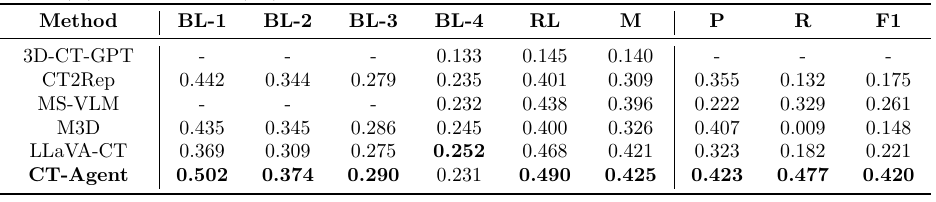
• Shows improvement? Still pretty bad; the CT2Rep baseline is again SIGNIFICANTLY WORSE than what’s reported in the original paper

• The regionally prompted analysis is by far the most interesting part, which shows that the agent either doesn’t know or can’t identify some organs well…
  • Surprisingly, bone is hard?

MedRegion-CT

Takeaway

An interesting way to “manage” contexts for an MLLM, though the benefits are limited

Method

Input:
The global visual information is provided here: <image>.
The following regions of interest have been identified: lung<region1>,
airway <region2>, .... abdomen <region6>
Additional clinical attribute information is provided as follows:
Organ Volumes:
Lung:

- Right Upper Lobe:{right_upper_lobe_volume}ml
- Right Middle Lobe:{right_middle_lobe_volume}m
  Right Lower Lobe:{right_lower_lobe_volume}ml
- Left Upper Lobe:{left_upper_lobe_volume}ml
- Left Lower Lobe:{left_lower_lobe_volume}m
  Heart:
- Left Atrium:{left_atrium_volume}ml
- Right Atrium:{right_atrium_volume}ml
  Left Ventricle:{left_ventricle_volume}ml
- Right Ventricle:{right_ventricle_volume}ml
  Liver:{liver_volume}ml
  Kidney:
- Left:{left_kidney_volume}ml
  Right:{right_kidney_volume}ml
  Lesion Details:
  Nodule:
- count:{nodule_count}
  diameter (mm):{nodule_diameter}
  location:{nodule_location}
  Cyst:
  count:{cyst_count}
  diameter (mm):{cyst_diameter}
- location:{cyst_location}
  Effusion:
  count:{effusion_count}
  diameter (mm):{effusion_diameter}
- location:{effusion_location}
  Describe this medical scan with findings.

Output:
[Lung]:{lung_findings]
[Airways]: {airways_findings]
[Mediastinum]: {mediastinum_findings}
[Heart]:{heart_findings]
[Osseous]:{osseous_findings]
[Abdomen]:{abdomen_findings}

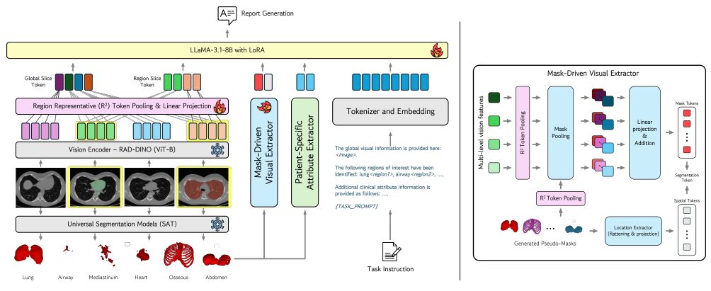
1. Leverage a pre-trained 2D Vision encoder (RAD-DINO) and heuristics to train global slice and region slice tokens
2. Leverage a 3D segmentation model (SAT) and add masks of 6 major organs and attributes (size of organ and lesions)

full setup:

Result

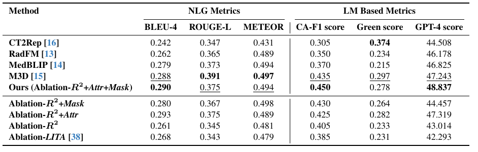
• Minor improvements over NLG metrics
• Greater degradation in the Green score may suggest a loss of medical findings…